SPT Graph
Tab
Interactive depth-based charts for SPT parameters with synchronized tooltips.
Tab Overview
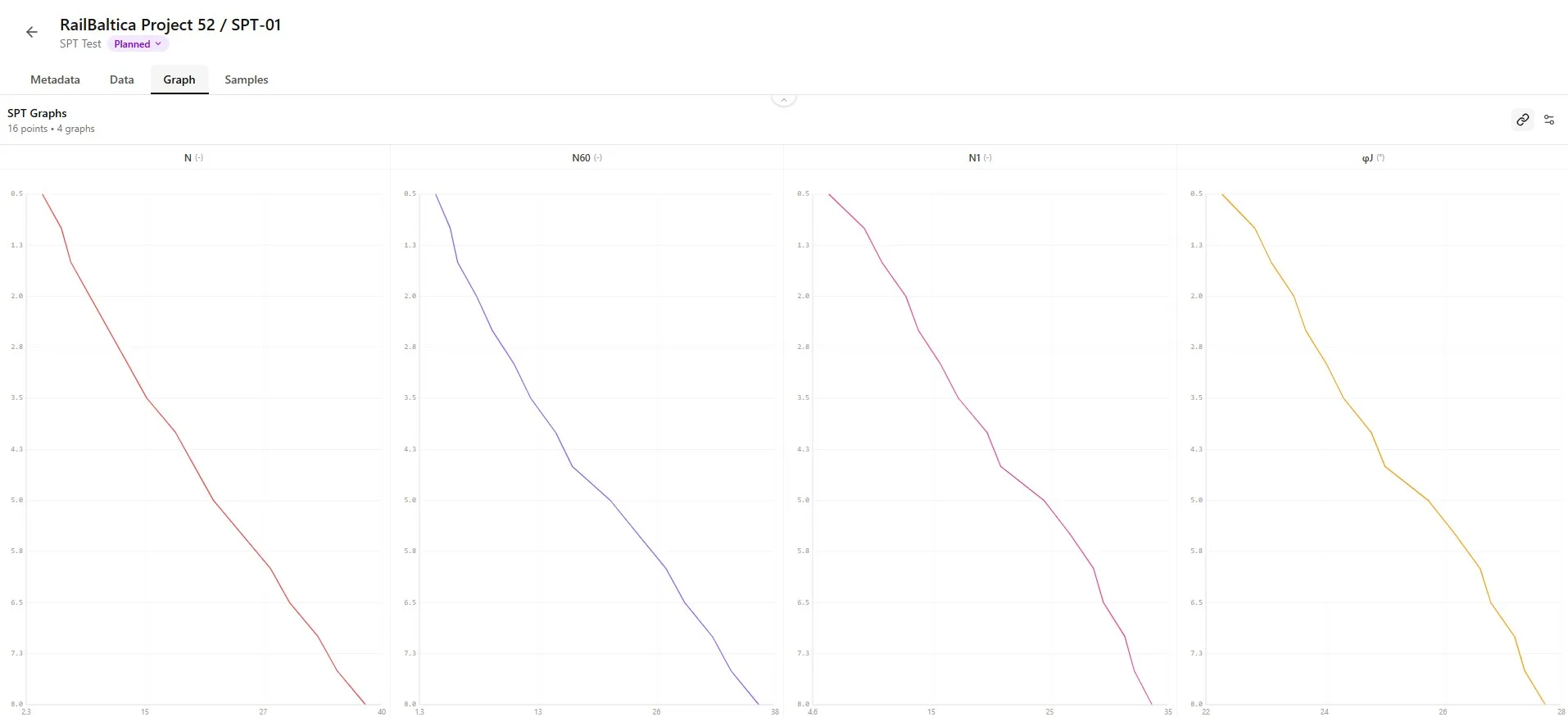
The SPT Graph tab visualizes raw measurements and calculated parameters as depth-based curves. Use it to spot trends, anomalies, and stiff/soft transitions across the borehole.
- Header — title and quick actions for the active SPT object.
- Toolbar — tooltip mode, settings, and pin controls.
- Settings panel — choose which graphs to display.
- Graph area — interactive depth-based charts with synchronized scroll.
Available Graphs
Borebase exposes three families of graphs: raw blow counts, depth-corrected values, and derived engineering parameters.
Raw Measurements
| Parameter | Unit | Color | Description |
|---|---|---|---|
| N — raw blow count (N2 + N3). | |||
| N2 — blow count for the second 15 cm interval. | |||
| N3 — blow count for the third 15 cm interval. | |||
| N1c — corrected raw blow count. |
Calculated Values
| Parameter | Unit | Color | Description |
|---|---|---|---|
| N60 — N standardized to 60 % energy ratio. | |||
| N1 — overburden-corrected N value. | |||
| σv — total vertical stress. | |||
| σ'v — effective vertical stress. | |||
| u — pore water pressure. |
Engineering Parameters
| Parameter | Unit | Color | Description |
|---|---|---|---|
| qc(SPT) — equivalent CPT cone resistance from SPT. | |||
| φ' (Jamiolkowski) — friction angle, Jamiolkowski correlation. | |||
| φ' (Hatanaka) — friction angle, Hatanaka & Uchida correlation. | |||
| φ' (Wolff) — friction angle, Wolff/Peck correlation. | |||
| Dr (Kulhawy & Mayne) — relative density correlation. | |||
| Dr (Skempton) — relative density correlation. | |||
| Es — Young's modulus estimate. | |||
| Es,max — maximum Young's modulus estimate. | |||
| qa — allowable bearing pressure estimate. |
Default Selection
By default the most useful graphs (N, N60, friction angle) are pre-selected so you see results immediately.Selecting Graphs to Display
Click the settings button in the toolbar to open the graph selection panel.

Toggle the checkboxes to add or remove graphs. The panel groups parameters by category.

- Color swatch — matches the line color used in the chart.
- Filled checkbox — graph is currently displayed.
- Close the panel to return to the graphs.
- Selections are saved automatically per object.
Practical Example
Showing only N60 and friction angle helps when preparing a foundation report — irrelevant raw curves are hidden.Tooltip Modes
Hovering a graph reveals depth-aligned values. Two modes control how tooltips behave across charts.
Synchronized Mode
Synchronized mode shows tooltips for the same depth across every visible graph at once — best for cross-parameter analysis.


Single Mode
Single mode shows the tooltip only for the chart under the cursor — best for focused inspection.

Tooltip Contents
Tooltips display the depth, raw value, calculated value, and applicable units.Pinning Data Points
Pin specific depths to keep their values visible while you continue scrolling and comparing.
- Click a point on any chart to pin it.
- Pin multiple depths at once for direct comparison.
- Pins persist until you clear them or leave the object.
- Pinning a depth marks that depth across all visible charts in sync mode.
Clearing Pinned Points
Use the clear button in the toolbar to remove all pinned points in one click.

Practical Example
Pin the depth of a soft clay lens and a dense sand layer to compare N60 side by side.Graph Features
Each chart shares a common layout for fast scanning.
- Title — parameter name and unit.
- Depth axis (Y) — synchronized across all charts.
- Value axis (X) — scaled to the parameter range.
- Grid lines aid visual reading at depth.
- Line color matches the legend in the settings panel.
- Horizontal scroll appears when many graphs are selected.
Empty Graphs
Calculated graphs require the underlying parameters to be present. Missing inputs leave the chart empty.
Data Required
Make sure metadata (energy ratio, rod length, sampler type) and water level are filled in — they drive N60 and stress-based calculations.Best Practices
Data Quality Checks
- Inspect raw N values for obviously erroneous spikes before relying on derived parameters.
- Confirm hammer energy and equipment corrections look reasonable in the Metadata tab.
- Cross-check stratigraphy boundaries against changes in N60.
- Pin suspicious points to revisit them after re-checking the field log.
Geotechnical Analysis
- Use friction angle correlations only within their documented validity range.
- Compare N1 with stratigraphy to confirm density trends with depth.
- Apply local experience when correlations disagree.
- Document which correlation you used in the final report.
Settlement Analysis
- Use Es and Es,max graphs together to bracket settlement estimates.
- Watch for sudden modulus changes that may indicate layer boundaries.
- Validate allowable bearing pressure against your settlement criterion.