SPT Data Tab
Deep Dive
Import, view, and analyze Standard Penetration Test data. Automatic N60 corrections, friction angle calculations using multiple methods, and engineering parameter estimation.
Interface Overview
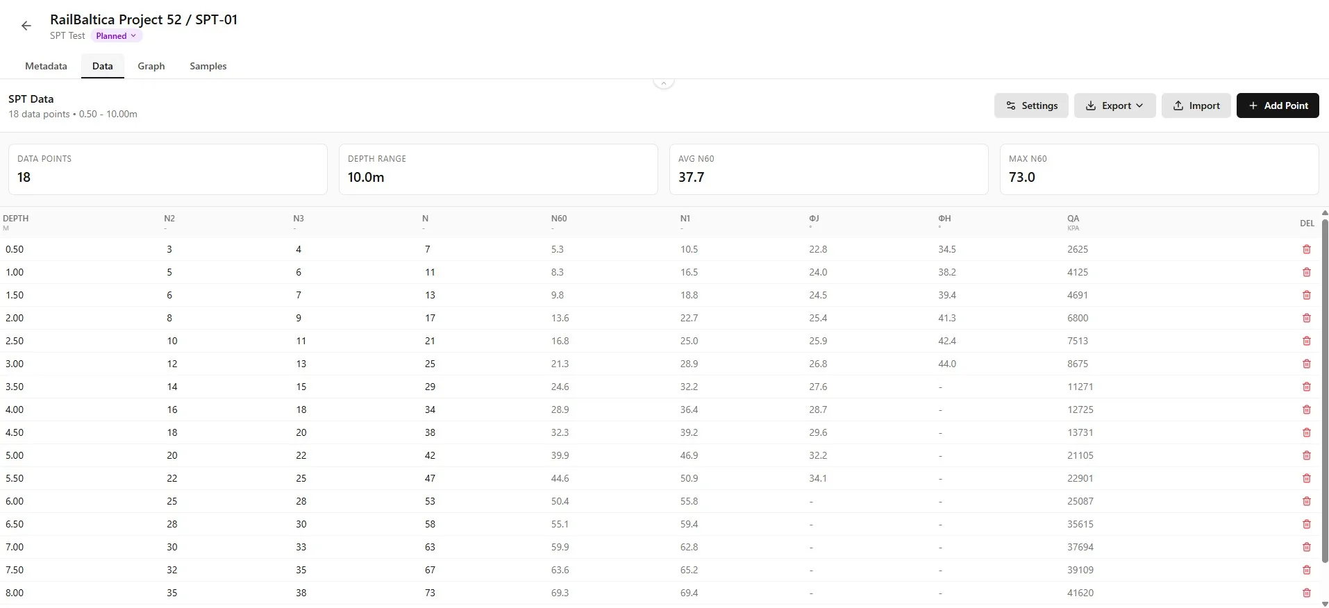
The SPT Data tab provides comprehensive data management with industry-standard corrections:
- Data point count, depth range, and action buttons (Settings, Export, Import, Add Point).
- Equipment parameters (borehole diameter, sampler type, hammer energy) and column visibility toggles.
- Quick statistics: data points count, depth range, average N, maximum N.
- Full data grid with blow counts, corrections, and engineering parameters.
Equipment Parameters
Before analyzing SPT data, configure the equipment parameters that affect correction factors:
Borehole Parameters
| Parameter | Options | Correction |
|---|---|---|
| 65-115 mm | Standard | 1.00 |
| 150 mm | Larger | 1.05 |
| 200 mm | Large | 1.15 |
Sampler Type
| Type | Description | Correction |
|---|---|---|
| Standard sampler | With liner | 1.10 |
| Sampler without liner | Dense sand, clay | 1.00 |
| Sampler without liner | Loose sand | 1.00 |
Rod Length Correction (CR)
| Rod Length Correction (CR) | Correction |
|---|---|
| < 3 m | 0.75 |
| 3 ≤ L < 4 m | 0.80 |
| 4 ≤ L < 6 m | 0.85 |
| 6 ≤ L < 10 m | 0.95 |
| ≥ 10 m | 1.00 |
Open the Metadata tab to review the SPT type and equipment settings.

In edit mode, check the SPT type, hammer weight, drop height, rod length, borehole diameter and whether a plastic liner is used. Save the settings for this test.

Understanding Data Columns
Data columns are organized into four categories:
Blow Counts (Editable)
| Column | Unit | Description |
|---|---|---|
| Depth | m | Test depth from surface |
| N1c | - | Calibration blows (first 15 cm, seating) |
| N2 | - | Second 15 cm blow count |
| N3 | - | Third 15 cm blow count |
| N | - | Total N value (N2 + N3) |
| ER | % | Energy ratio (default 60%) |
Soil Parameters (Editable)
| Column | Unit | Description |
|---|---|---|
| γd | kN/m³ | Dry unit weight of soil |
| γsat | kN/m³ | Saturated unit weight of soil |
| Soil Type | - | Select from stratigraphy layers |
Corrected Values (Read-Only)
| Column | Unit | Description |
|---|---|---|
| N60 | - | Energy-corrected N value (N × ER/60) |
| Hd | m | Height of dry soil column |
| Hs | m | Height of saturated soil column |
| σv | kPa | Total vertical stress |
| u | kPa | Pore water pressure |
| σ'v | kPa | Effective vertical stress |
Engineering Parameters (Read-Only)
| Column | Unit | Description |
|---|---|---|
| N1 | - | Overburden-corrected N60 |
| qc | MPa | CPT equivalent cone resistance |
| φJ | ° | Friction angle (Jamiolkowski method) |
| φH | ° | Friction angle (Hatanaka-Uchida) |
| φW | ° | Friction angle (Wolff method) |
| DrKM | % | Relative density (Kulhawy & Mayne) |
| DrS | % | Relative density (Skempton) |
| Es | MPa | Minimum elastic modulus |
| Esmax | MPa | Maximum elastic modulus |
| qa | kPa | Ultimate bearing capacity |
N60 Energy Correction
The N60 value normalizes SPT blow counts to 60% energy efficiency:
| Factor | Description |
|---|---|
| ER | Energy ratio of hammer (typically 45-80%) |
| CB | Borehole diameter correction |
| CS | Sampler type correction |
| CR | Rod length correction |
Friction Angle Calculations
Borebase calculates friction angle using three established methods:
Jamiolkowski et al. (1988)
Best for normally consolidated sands. Uses overburden-corrected N value.
Hatanaka & Uchida (1996)
Widely used correlation for granular soils. Simple and reliable.
Wolff (1989)
Uses the overburden-corrected N1 value to estimate the friction angle.
Relative Density Estimation
Two methods for estimating relative density of granular soils:
Kulhawy & Mayne (1990)
Uses overburden-corrected N1 value. Suitable for clean sands.
Skempton (1986)
Accounts for vertical effective stress. Coefficients a and b depend on soil type.
- Very Loose
- Loose
- Medium Dense
- Dense
- Very Dense
Elastic Modulus Estimation
The elastic modulus range is estimated from N1 values:
Importing SPT Data
Import SPT data from CSV or Excel files:
Click Import in the Data tab toolbar to open the import wizard.

Drop your CSV or Excel file into the upload area, or click Select File to choose it.

The wizard attempts to detect the columns automatically. Review the detected fields and any warnings before continuing.

Set the first data row so that header rows are skipped. Check the depth unit, water level and, for CSV files, the delimiter and decimal separator.

Map the depth column and either N2 plus N3 or N Total. Map optional fields such as energy ratio, unit weights and soil type when they are present.

Review the data preview and warnings. Check whether Replace Existing Data is selected, as this option replaces the current measurements.

Click Import after checking the displayed point count. Wait for the result, then review any reported errors.

Soil Type Selection
Link SPT data points to stratigraphy layers for automatic unit weight assignment:
- Click the Soil Type dropdown for any data row.
- Select from available stratigraphy layers defined in the Strata tab.
- Unit weights (γ dry, γ sat) are automatically populated from the layer properties.
- All stress calculations update automatically.
Adding a Data Point
You can add individual SPT measurements manually in the Data tab.
Click Add Point in the toolbar to open the entry form.

Enter the depth and the available blow counts (N2, N3 or N Total). Add unit weights and a soil type if available, then click Add.

Settings
Click Settings in the Data tab toolbar to open calculation and display settings.

Under Calculation Parameters, set the water level and click Apply & Recalculate to update the calculated values.

Under Visible Columns, expand Raw, Calculated or Engineering and select the columns to show in the table.

Select Export only visible columns to include only the displayed columns in CSV and Excel exports. Clear it to export all available columns.

Exporting SPT Data
Export your SPT data with all calculations for reports:
Click Export in the Data tab toolbar.

Choose Export CSV or Export Excel to download the data in the selected format.

- All visible columns in comma-separated format. Open in Excel, Python, or any data tool.
- Professional formatting with styled headers, proper column widths, and formulas preserved.
Best Practices
Data Entry
- Always enter the calibration blows (N1c) even though they're not used in N calculation.
- Verify energy ratio with your testing equipment - don't assume 60%.
- Link data points to stratigraphy layers for consistent unit weights.
Quality Control
- Watch for refusal values (N > 50) which may indicate hitting bedrock or very dense layers.
- Check for unit weight warnings (yellow triangle icons).
- Compare friction angles from different methods - large discrepancies may indicate issues.
Interpretation
- SPT correlations work best for sands and gravels. Use caution with clays.
- Consider using the conservative (lower) friction angle for design.
- Elastic modulus ranges are wide - use laboratory tests for important projects.